Tag Archives: performance

Microservices in C# Part 5: Autoscaling

Balancing demand and processing power

Autoscaling Microservices

In the previous tutorial, we demonstrated the throughput increase by invoking multiple instances of SimpleMathMicroservice, in order to facilitate a greater number of concurrent inbound HTTP requests. We experimented with various configurations, increasing the count of simultaneously running instances of SimpleMathMicroservice until the law of diminishing returns set it.

This is a perfectly adequate configuration for applications that absorb a consistent number of inbound HTTP requests over any given extended period of time. Most web applications, of course, do not adhere to this model. Instead, traffic tends to fluctuate, depending on several factors, not least of which is the type of business that the web application facilitates.

This presents a significant problem, in that we cannot manually throttle the number of concurrently running Microservice instances on-demand, as traffic dictates. We need an automated mechanism to scale our Microservice instances adequately.

Autoscaling involves more than simply increasing the count of running instances during heavy load. It also involves the graceful termination of superfluous instances, or instances that are no longer necessary to meet the demands of the application as load is reduced. Daishi.AMQP provides just such features, which we’ll cover in detail.

QueueWatch

QueueWatch is a mechanism that allows the monitoring of RabbitMQ Queues in real time. It achieves this by polling the RabbitMQ Management API (mentioned in Part #3) at regular intervals, returning metadata that describes the current state of each Queue.

Metadata

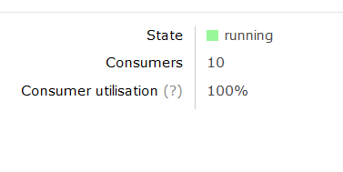
RabbitMQ exposes important metadata pertaining to each Queue. This metadata is presented in a user-friendly manner in the RabbitMQ Management Console:

Message Rates

These metrics represent the rates at which messages are processed by RabbitMQ. “Publish” illustrates the rate at which messages are introduced to the server, while “Deliver” represents the rate at which messages are dispatched to listening consumers (Microservices, in our case).

This information is readily available in the RabbitMQ Management API. QueueWatch effectively harvests this information, comparing the values retrieved in the latest poll with those retrieved in the previous, to monitor the flow of messages through RabbitMQ. QueueWatch can determine whether or not any given Queue is idling, overworked, or somewhere in between.

Once a Queue is determined to be under heavy load, QueueWatch triggers an event, and dispatches an AutoScale message to the Microservice consuming the heavily-laden Queue. The Microservice can then instantiate more AMQPConsumer instances in order to drain the Queue sufficiently.

Just Show Me the Code

Create a new Microservice instance called QueueWatchMicroservice; an implementation of Microservice, and add the following code to the Init method:

            var amqpQueueMetricsManager = new RabbitMQQueueMetricsManager(false, "localhost", 15672, "paul", "password");

            AMQPQueueMetricsAnalyser amqpQueueMetricsAnalyser = new RabbitMQQueueMetricsAnalyser(
                new ConsumerUtilisationTooLowAMQPQueueMetricAnalyser(
                    new ConsumptionRateIncreasedAMQPQueueMetricAnalyser(
                        new DispatchRateDecreasedAMQPQueueMetricAnalyser(
                            new QueueLengthIncreasedAMQPQueueMetricAnalyser(
                                new ConsumptionRateDecreasedAMQPQueueMetricAnalyser(
                                    new StableAMQPQueueMetricAnalyser()))))), 20);

            AMQPConsumerNotifier amqpConsumerNotifier = new RabbitMQConsumerNotifier(RabbitMQAdapter.Instance, "monitor");
            RabbitMQAdapter.Instance.Init("localhost", 5672, "paul", "password", 50);

            _queueWatch = new QueueWatch(amqpQueueMetricsManager, amqpQueueMetricsAnalyser, amqpConsumerNotifier, 5000);
            _queueWatch.AMQPQueueMetricsAnalysed += QueueWatchOnAMQPQueueMetricsAnalysed;

            _queueWatch.StartAsync();

There’s a lot to talk about here. Firstly, remember that the primary function of QueueWatch is to poll the RabbitMQ Management API. In doing so, QueueWatch returns several metrics pertaining to each Queue. We need to decide which metrics we are interested in.

Metrics are represented by implementations of AMQPQueueMetricAnalyser, and chained together as per the Chain of Responsibility Design Pattern. Each link in the chain is executed until a predefined performance condition is met. For example, let’s consider the ConsumerUtilisationTooLowAMQPQueueMetricAnalyser. This implementation of AMQPQueueMetricAnalyser inspects the ConsumerUtilisation metric, and determines whether the value is less than 99%, in which case, there are not enough consuming Microservices to adequately drain the Queue. At this point, a ConsumerUtilisationTooLow value is returned, the chain of execution ends, and QueueWatch issues an AutoScale directive:

        public override void Analyse(AMQPQueueMetric current, AMQPQueueMetric previous, ConcurrentBag<AMQPQueueMetric> busyQueues, ConcurrentBag<AMQPQueueMetric> quietQueues, int percentageDifference) {
            if (current.ConsumerUtilisation >= 0 && current.ConsumerUtilisation < 99) {
                current.AMQPQueueMetricAnalysisResult = AMQPQueueMetricAnalysisResult.ConsumerUtilisationTooLow;
                busyQueues.Add(current);
            }
            else analyser.Analyse(current, previous, busyQueues, quietQueues, percentageDifference);
        }

Scale-Out Directive

Scaling out

QueueWatch must issue Scale-Out directives through dedicated Queues in order to adhere to the Decoupled Middleware design. QueueWatch should not know anything about the downstream Microservices, and should instead communicate through AMQP, specifically, through a dedicated Exchange.

Each Microservice must now listen to 2 Queues. E.g., SimpleMathMicroservice will continue listening to the Math Queue, as well as a Queue called AutoScale, for the purpose of demonstration. SimpleMathMicroservice will receive Scale-Out directives through this Queue. We should modify SimpleMathMicroservice accordingly:

        public void Init() {
            _adapter = RabbitMQAdapter.Instance;
            _adapter.Init("localhost", 5672, "guest", "guest", 50);

            _rabbitMQConsumerCatchAll = new RabbitMQConsumerCatchAll("Math", 10);
            _rabbitMQConsumerCatchAll.MessageReceived += OnMessageReceived;

            _autoScaleConsumerCatchAll = new RabbitMQConsumerCatchAll("AutoScale", 10);
            _autoScaleConsumerCatchAll.MessageReceived += _autoScaleConsumerCatchAll_MessageReceived;

            _consumers.Add(_rabbitMQConsumerCatchAll);

            _adapter.Connect();
            _adapter.ConsumeAsync(_autoScaleConsumerCatchAll);
            _adapter.ConsumeAsync(_rabbitMQConsumerCatchAll);
        }

Create a Topic Exchange called “monitor”. QueueWatch will publish to this Exchange, which will route the message to an appropriate Queue. Now create a binding between the monitor Exchange and the AutoScale Queue:

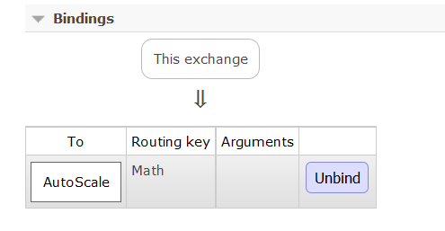
Exchange Binding

Note that the Routing Key is the name of the Queue under monitor. If QueueWatch determines that the Math Queue is under load, then it will issue a Scale-Out directive to the monitor Exchange, with a Routing Key of “Math”. The monitor Exchange will react by routing the Scale-Out directive to the AutoScale Queue, to which an explicit binding exists. SimpleMathMicroservice consumes the Scale-Out directive and reacts appropriately, by instantiating a new AMQPConsumer:

            if (e.Message.Contains("scale-out")) {
                var consumer = new RabbitMQConsumerCatchAll("Math", 10);
                _adapter.ConsumeAsync(consumer);
                _consumers.Add(consumer);
            }
            else {
                if (_consumers.Count <= 1) return;
                var lastConsumer = _consumers[_consumers.Count - 1];

                _adapter.StopConsumingAsync(lastConsumer);
                _consumers.RemoveAt(_consumers.Count - 1);
            }

Summary

QueueWatch provides a means of returning key RabbitMQ Queue metrics at regular intervals, in order to determine whether demand, in terms of the number of running Microservice instances, is waxing or waning. QueueWatch also provides a means of reacting to such events, by publishing AutoScale notifications to downstream Microservices, so that they can scale accordingly, providing sufficient processing power at any given instant. The process is simplified as follows:

QueueWatch returns metrics describing each Queue
Queue metrics are compared against the last batch returned by QueueWatch
AutoScale messages are dispatched to a Monitor Exchange
AutoScale messages are routed to the appropriate Queue
AutoScale messages are consumed by the intended Microservices
Microservices scale appropriately, based on the AutoScale message

Next Steps

Prevent a “bounce” effect as traffic arbitrarily fluctuates for reasons not pertaining to application usage, such as network slow-down, or hardware failure
The current implementation compares metrics in a very simple fashion. Future implementations will instead graph metric metadata, and react to more thoroughly defined thresholds

Connect with me:

Microservices in C# Part 4: Scaling Out

Leave a reply

Scaling out our Microservices

So far, we have

established a simple Microservice
abstracted and sufficiently covered the Microservice core logic in terms of tests
created a reusable Microservice template
implemented the queue-pooling concept to ensure reliable message delivery
run simple load tests to adequately size Queue resources

Now it’s time to scale out. Here’s how our design currently looks:

Our current design

This design is fine for demonstration purposes, but requires augmentation to facilitate production release. Consider that the current design will only service a single request at any given time, and will service requests in a FIFO manner, assuming that no hardware failure, or otherwise, occurs.

Even under ideal conditions, assuming that each request takes exactly 1 second to complete, given 100 inbound HTTP requests, the 1st request will complete in 1 second. The final, 100th request, will complete in 100 seconds.

Clearly, this is less than ideal. Intuitively, we might consider optimising the processing speed of our Microservice. Certainly this will help, but does little to solve the problem. Let’s say that our engineers work tirelessly to cut response times in half:

Working tirelessly to shatter response-times!

Even if they achieve this, in a batch of 100 requests, the 100th request will still take 50 seconds to complete. Instead, let’s focus on serving multiple requests in a concurrent, and potentially parallel manner. Our augmented design will be as follows:

Augmented design

Notice that instead of a single instance of SimpleMathMicroservice, there are now multiple instances running. How many instances do we need? That depends on 2 factors – response times and something called Quality-of-Service (QOS).

Quality of Service

Quality of Service is a feature of AMQP that defines the level of service exhibited by AMQP Channels at any given time. QOS is expressed as a percentage; 100% suggests that any given channel is utilised to maximum effect. Essentially, we need to avoid downtime in terms of channel-usage. Downtime can be described as the period of time that a Microservice is idle, or not doing work.

Typically, such scenarios occur when a Microservice is waiting on messages in transit, or is itself transmitting message-receipt acknowledgements to the Message Bus. For more information on QOS, please refer to this post. For the moment, we’re going to begin with the most intuitive design possible, without delving deeply into the complexities of QOS, and related concepts such as prefetch-count.

To that end, we are going to deploy multiple instances of our SimpleMathMicroservice (10, to be exact), and retain the default message-delivery mechanism – to read each message from a Queue one-at-a-time. In order to achieve this, we must modify our application slightly, specifically, the Global.asax.cs file. First, add a simple collection to house multiple running SimpleMathMicroservice instances:

private readonly List<SimpleMathMicroservice> _simpleMathMicroservices = new List<SimpleMathMicroservice>();

Now, instantiate 10 unique instances of SimpleMathMicroservice, initialise each instance, and add it to the collection:

            for (var i = 0; i < 10; i++) {
                var simpleMathMicroservice = new SimpleMathMicroservice();
                _simpleMathMicroservices.Add(simpleMathMicroservice);

                simpleMathMicroservice.Init();
            }

Finally, modify the Application_End function such that it gracefully shuts down each SimpleMathMicroservice instance:

            foreach (var simpleMathMicroservice in _simpleMathMicroservices) {
                simpleMathMicroservice.Shutdown();
            }

Now, on startup, 10 instances of SimpleMathMicroservice will be invoked, and will each actively listen to the Math Queue.

Message Distribution

SimpleMathMicroservice leverages a component called AMQPConsumer within the Daishi.AMQP library that defines the manner in which SimpleMathMicroservice will read messages from any given Queue. AMQPConsumer exposes a constructor that accepts a value called prefetchCount:

        protected AMQPConsumer(string queueName, int timeout, ushort prefetchCount = 1, bool noAck = false,
            bool createQueue = true, bool implicitAck = true, IDictionary<string, object> queueArgs = null) {
            this.queueName = queueName;
            this.prefetchCount = prefetchCount;
            this.noAck = noAck;
            this.createQueue = createQueue;
            this.timeout = timeout;
            this.implicitAck = implicitAck;
            this.queueArgs = queueArgs;
        }

Notice the default prefetchCount value of 1. This default setting results behaviour that allows the component to read messages one-at-a-time. It also ensures that RabbitMQ will distribute messages evenly, in a round-robin manner, among consumers. Now our application is configured to process multiple requests in a concurrent manner.

Concurrency and Parallelism

Can our application now be described a parallel? That depends. Concurrency is essentially the act of performing multiple tasks on a single CPU, or core. Parallelism on the other hand, can be described as the act of performing multiple tasks, or multiple stages of a single task, across multiple cores.

By this definition, or application certainly operates in a concurrent manner. But does it also operate in a parallel manner? That depends. Running the application on a single core machine obviously prohibits parallelism. Running on multiple cores will very likely result in parallel processing. Under the hood, the Daishi.AMQP library invokes a new thread for each Microservice operation that consumes messages from a Queue:

        public void ConsumeAsync(AMQPConsumer consumer) {
            if (!IsConnected) Connect();

            var thread = new Thread(o => consumer.Start(this));
            thread.Start();

            while (!thread.IsAlive)
                Thread.Sleep(1);
        }

“Wait, you shouldn’t invoke threads manually! That’s what ThreadPool.QueueUserWorkItem() is for!”

ThreadPool.QueueUserWorkItem() invokes threads as background operations. We require foreground threads, to ensure that the OS provides enough resources to run sufficiently, and also to prevent the OS from pre-empting the thread altogether, in cases when heavy load reduces resource availability.

Assuming that batches of newly created threads run (or are context-switched) across multiple cores, one could argue that our application exhibits parallel processing behaviour.

Run an ApacheBench load test against the running application:

ab -n 10000 -c 10 http://localhost:46653/api/math/1500

While the test is running, refer to the Math Queue in the RabbitMQ Administrator interface:

http://localhost:15672/#/queues/%2F/Math

Notice the number of Consumers (10) and the Consumer Utilisation figure. This figure represents the QOS value associated with the Queue. It should settle at the 100% mark for the duration of the test, indicating that each of all 10 SimpleMathMicroservice instances are constantly busy, and not idle:

Quality of Service

Next Steps

Modify the number of running SimpleMathMicroservice instances, and apply load tests to each setting. Ideally, push the number of running instances upwards in reasonable increments (batches of 5-10) and observe the response times, comparing each run against the last.

Response times should improve incrementally, then plateau, and ultimately decrease as you increase the number of running instances. This is an indication that your application has reach critical mass, based on the law of diminishing returns. Doing this will yield the number of SimpleMathMicroservice instances that you should deploy in order to achieve optimal throughput.

Connect with me:

Microservices in C# Part 3: Queue Pool Sizing

Leave a reply

Fine tuning QueuePool

This tutorial expands on the previous tutorial, focusing on the Queue Pool concept. By way of quick refresher, a Queue Pool is a feature of the Daishi.AMQP library that allows AMQP Queues to be shared among clients in a concurrent capacity, such that each Queue will have 0…1 consumers only. The concept is not unlike database connection-pooling.

We’ve built a small application that leverages a simple downstream Microservice, implements the AMQP protocol over RabbitMQ, and operates a QueuePool mechanism. We have seen how the QueuePool can retrieve the next available Queue:

var queue = QueuePool.Instance.Get();

And how Queues can be returned to the QueuePool:

QueuePool.Instance.Put(queue);

We have also considered the QueuePool default Constructor, how it leverages the RabbitMQ Management API to return a list of relevant Queues:

        private QueuePool(Func&amp;lt;AMQPQueue&amp;gt; amqpQueueGenerator) {
            _amqpQueueGenerator = amqpQueueGenerator;
            _amqpQueues = new ConcurrentBag&amp;lt;AMQPQueue&amp;gt;();

            var manager = new RabbitMQQueueMetricsManager(false, &amp;quot;localhost&amp;quot;, 15672, &amp;quot;paul&amp;quot;, &amp;quot;password&amp;quot;);
            var queueMetrics = manager.GetAMQPQueueMetrics();

            foreach (var queueMetric in queueMetrics.Values) {
                Guid queueName;
                var isGuid = Guid.TryParse(queueMetric.QueueName, out queueName);

                if (isGuid) {
                    _amqpQueues.Add(new RabbitMQQueue {IsNew = false, Name = queueName.ToString()});
                }
            }
        }

Notice the high-order function in the above constructor. In the QueuePool static Constructor we define this function as follows:

        private static readonly QueuePool _instance = new QueuePool(
            () =&amp;gt; new RabbitMQQueue {
                Name = Guid.NewGuid().ToString(),
                IsNew = true
            });

This function will be invoked if the QueuePool is exhausted, and there are no available Queues. It is a simple function that creates a new RabbitMQQueue object. The Daishi.AMQP library will ensure that this Queue is created (if it does not already exist) when referenced.

Exhaustion is Expensive

QueuePool exhaustion is something that we need to avoid. If our application frequently consumes all available Queues then the QueuePool will become ineffective. Let’s look at how we go about avoiding this scenario.

First, we need some targets. We need to know how much traffic our application will absorb in order to adequately size our resources. For argument’s sake, let’s assume that our MathController will be subjected to 100,000 inbound HTTP requests, delivered in batches of 10. In other words, at any given time, MathController will service 10 simultaneous requests, and will continue doing so until 100,000 requests have been served.

Stress Testing Using Apache Bench

Apache Bench is a very simple, lightweight tool designed to test web-based applications, and is bundled as part of the Apache Framework. Click here for simple download instructions. Assuming that our application runs on port 46653, here is the appropriate Apache Bench command to invoke 100 MathController HTTP requests in batches of 10:

-ab -n 100 -c 10 http://localhost:46653/api/math/150

Notice the “n” and “c” paramters; “n” refers to “number”, as in the number of requests, and “c” refers to “concurrency”, or the amount of requests to run in simultanously. Running this command will yield something along the lines of the following:
Benchmarking localhost (be patient).....done

Server Software: Microsoft-IIS/10.0
Server Hostname: localhost
Server Port: 46653

Document Path: /api/math/150
Document Length: 5 bytes

Concurrency Level: 10
Time taken for tests: 7.537 seconds
Complete requests: 100
Failed requests: 0
Total transferred: 39500 bytes
HTML transferred: 500 bytes
Requests per second: 13.27 [#/sec] (mean)
Time per request: 753.675 [ms] (mean)
Time per request: 75.368 [ms] (mean, across all concurrent requests)
Transfer rate: 5.12 [Kbytes/sec] received

Connection Times (ms)
min mean[+/-sd] median max
Connect: 0 0 0.4 0 1
Processing: 41 751 992.5 67 3063
Waiting: 41 751 992.5 67 3063
Total: 42 752 992.4 67 3063

Percentage of the requests served within a certain time (ms)
50% 67
66% 1024
75% 1091
80% 1992
90% 2140
95% 3058
98% 3061
99% 3063
100% 3063 (longest request)

Adjusting QueuePool for Optimal Results

Those results don’t look great. Incidentally, if you would like more information as regards how to interpret Apache Bench results, click here. Let’s focus on the final section, “Percentage of the requests served within a certain time (ms)”. Here we see that 75% of all requests took just over 1 second (1091 ms) to complete. 10% took over 2 seconds, and 5% took over 3 seconds to complete. That’s quite a long time for such a simple operation running on a local server. Let’s run the same command again:
Benchmarking localhost (be patient).....done

Server Software: Microsoft-IIS/10.0
Server Hostname: localhost
Server Port: 46653

Document Path: /api/math/100
Document Length: 5 bytes

Concurrency Level: 10
Time taken for tests: 0.562 seconds
Complete requests: 100
Failed requests: 0
Total transferred: 39500 bytes
HTML transferred: 500 bytes
Requests per second: 177.94 [#/sec] (mean)
Time per request: 56.200 [ms] (mean)
Time per request: 5.620 [ms] (mean, across all concurrent requests)
Transfer rate: 68.64 [Kbytes/sec] received

Connection Times (ms)
min mean[+/-sd] median max
Connect: 0 0 0.4 0 1
Processing: 29 54 11.9 49 101
Waiting: 29 53 11.9 49 101
Total: 29 54 11.9 49 101

Percentage of the requests served within a certain time (ms)
50% 49
66% 54
75% 57
80% 60
90% 73
95% 80
98% 94
99% 101
100% 101 (longest request)

OK. Those results look a lot better. Even the longest request took 101 ms, and 80% of all requests completed in <= 60 ms.

But where does this discrepancy come from? Remember, that on start-up there are no QueuePool Queues. The QueuePool is empty and does not have any resources to distribute. Therefore, inbound requests force QueuePool to create a new Queue in order to facilitate the request, and then reclaim that Queue when the request has completed.

Does this mean that when I deploy my application, the first batch of requests are going to run much more slowly than subsequent requests?

No, that’s where sizing comes in. As with all performance testing, the objective is to set a benchmark in terms of the expected volume that an application will absorb, and to determine that maximum impact that it can withstand, in terms of traffic. In order to sufficiently bootstrap QueuePool, so that it contains an adequate number of dispensable Queues, we can simply include ASP.NET controllers that leverage QueuePool in our performance run.

Suppose that we expect to handle 100 concurrent users over extended periods of time. Let’s run an Apache Bench command again, setting the level of concurrency to 100, with a suitably high number of requests in order to sustain that volume over a reasonably long period of time:

ab -n 1000 -c 100 http://localhost:46653/api/math/100

Percentage of the requests served within a certain time (ms) 50% 861 66% 938 75% 9560 80% 20802 90% 32949 95% 34748 98% 39756 99% 41071 100% 42163 (longest request)
Again, very poor, but expected results. More interesting is the number of Queues now active in RabbitMQ:

New QueuePool Queues

In my own environment, QueuePool created 100 Queues in order to facilitate all inbound requests. Let’s run the test again, and consider the results:
Percentage of the requests served within a certain time (ms) 50% 497 66% 540 75% 575 80% 591 90% 663 95% 689 98% 767 99% 816 100% 894 (longest request)
These results are much more respectable. Again, the discrepancy between performance runs is due to the fact that QueuePool was not adequately initialised during the first run. However, QueuePool was initialised with 100 Queues, a volume sufficient to facilitate the volume of request that the application is expected to serve. This is simple an example as possible.

Real world performance testing entails a lot more than simply executing isolated commands against single endpoints, however the principal remains the same. We have effectively determined the optimal size necessary for QueuePool to operate efficiently, and can now size it accordingly on application start-up, ensuring that all inbound requests are served quickly and without bias.

Those already versed in the area of Microservices might object at this point. There is only a single instance of our Microservice, SimpleMathMicroservice, running. One of the fundamental concepts behind Microservice design is scalability. In my next article, I’ll cover scaling, and we’ll drive those performance response times into the floor.

Connect with me:

Microservices in C# Part 2: Consistent Message Delivery

5 Replies

Microservice Architecture

Ensuring that Messages are Consumed by their Intended Recipient

This tutorial builds on the simple Microservice application that we built in the previous tutorial. Everything looks good so far, but what happens when we release this to production, and our application is consumed by multiple customers? Routing problems and message-correlation issue begin to rear their ugly heads. Our current example is simplistic. Consider a deployed application that performs work that is much more complex than our example.

Now we are faced with a problem; how to ensure that any given message is received by its intended recipient only. Consider the following process flow:

potential for mismatched message-routing

It is possible that outbound messages published from the SimpleMath Microservice may not arrive at the ASP.NET application in the same order in which the ASP.NET application initially published the corresponding request to the SimpleMath Microservice.

RabbitMQ has built-in safeguards against this scenario in the form of Correlation IDs. A Correlation ID is essentially a unique value assigned by the ASP.NET application to inbound messages, and retained throughout the entire process flow. Once processed by the SimpleMath Microservice, the Correlation ID is inserted into the associated response message, and published to the response Queue.

Upon receipt of any given message, the ASP.NET inspects the message contents, extracts the Correlation ID and compares it to the original Correlation ID. Consider the following pseudo-code:

            Message message = new Message();
            message.CorrelationID = new CorrelationID();

            RabbitMQAdapter.Instance.Publish(message.ToJson(), "MathInbound");

            string response;
            BasicDeliverEventArgs args;

            var responded = RabbitMQAdapter.Instance.TryGetNextMessage("MathOutbound", out response, out args, 5000);

            if (responded) {
                Message m = Parse(response);
                if (m.CorrelationID == message.CorrelationID) {
                    // This message is the intended response associated with the original request
                }
                else {
                    // This message is not the intended response, and is associated with a different request
                    // todo: Put this message back in the Queue so that its intended recipient may receive it...
                }
            }
            throw new HttpResponseException(HttpStatusCode.BadGateway);

What’s wrong with this solution?

It’s possible that any given message may be bounced around indefinitely, without ever reaching its intended recipient. Such a scenario is unlikely, but possible. Regardless, it is likely, given multiple Microservices, that messages will regularly be consumed by Microservices to whom the message was not intended to be delivered. This is an obvious inefficiency, and very difficult to control from a performance perspective, and impossible to predict in terms of scaling.

But this is the generally accepted solution. What else can we do?

An alternative, but discouraged solution is to invoke a dedicated Queue for each request:

dedicated queue per inbound request

Whoa! Are you suggesting that we create a new Queue for each request?!?

Yes, so let’s park that idea right there – it’s essentially a solution that won’t scale. We would place an unnecessary amount of pressure on RabbitMQ in order to fulfil this design. A new Queue for every inbound HTTP request is simply unmanageable.

Or, is it?

What if we could manage this? Imagine a dedicated pool of Queues, made available to inbound requests, such that each Queue was returned to the pool upon request completion. This might sound far-fetched, but this is essentially the way that database connection-pooling works. Here is the new flow:

consistent message routing using queue-pooling

Let’s walk through the code, starting with the QueuePool itself:

    public class QueuePool {
        private static readonly QueuePool _instance = new QueuePool(
            () => new RabbitMQQueue {
                Name = Guid.NewGuid().ToString(),
                IsNew = true
            });

        private readonly Func<AMQPQueue> _amqpQueueGenerator;
        private readonly ConcurrentBag<AMQPQueue> _amqpQueues;

        static QueuePool() {}

        public static QueuePool Instance { get { return _instance; } }

        private QueuePool(Func<AMQPQueue> amqpQueueGenerator) {
            _amqpQueueGenerator = amqpQueueGenerator;
            _amqpQueues = new ConcurrentBag<AMQPQueue>();

            var manager = new RabbitMQQueueMetricsManager(false, "localhost", 15672, "guest", "guest");
            var queueMetrics = manager.GetAMQPQueueMetrics();

            foreach (var queueMetric in queueMetrics.Values) {
                Guid queueName;
                var isGuid = Guid.TryParse(queueMetric.QueueName, out queueName);

                if (isGuid) {
                    _amqpQueues.Add(new RabbitMQQueue {IsNew = false, Name = queueName.ToString()});
                }
            }
        }

        public AMQPQueue Get() {
            AMQPQueue queue;

            var queueIsAvailable = _amqpQueues.TryTake(out queue);
            return queueIsAvailable ? queue : _amqpQueueGenerator();
        }

        public void Put(AMQPQueue queue) {
            _amqpQueues.Add(queue);
        }
    }

QueuePool is a static class that retains a reference to a synchronised collection of Queue objects. The most important aspect of this is that the collection is synchronised, and therefore thread-safe. Under the hood, incoming HTTP requests obtain mutually exclusive locks in order to extract a Queue from the collection. In other words, any given request that extracts a Queue is guaranteed to have exclusive access to that Queue.

Note the private constructor. Upon start-up (QueuePool will be initialised by the first inbound HTTP request) and will invoke a call to the RabbitMQ HTTP API, returning a list of all active Queues. You can mimic this call as follows:

curl -i -u guest:guest http://localhost:15672/api/queues

The list of returned Queue objects is filtered by name, such that only those Queues that are named in GUID-format are returned. QueuePool expects that all underlying Queues implement this convention in order to separate them from other Queues leveraged by the application.

Now we have a list of Queues that our QueuePool can distribute. Let’s take a look at our updated Math Controller:

            var queue = QueuePool.Instance.Get();
            RabbitMQAdapter.Instance.Publish(string.Concat(number, ",", queue.Name), "Math");

            string message;
            BasicDeliverEventArgs args;

            var responded = RabbitMQAdapter.Instance.TryGetNextMessage(queue.Name, out message, out args, 5000);
            QueuePool.Instance.Put(queue);

            if (responded) {
                return message;
            }
            throw new HttpResponseException(HttpStatusCode.BadGateway);

Let’s step through the process flow from the perspective of the ASP.NET application:

Retrieves exclusive use of the next available Queue from the QueuePool
Publishes the numeric input (as before) to SimpleMath Microservice, along with the Queue-name
Subscribes to the Queue retrieved from QueuePool, awaiting inbound messages
Receives the response from SimpleMath Microservice, which published to the Queue specified in step #2
Releases the Queue, which is re-inserted into QueuePool’s underlying collection

Notice the Get method. An attempt is made to retrieve the next available Queue. If all Queues are currently in use, QueuePool will create a new Queue.

Summary

Leveraging QueuePool offers greater reliability in terms of message delivery, as well as consistent throughput speeds, given that we no longer need rely on consuming components to re-queue messages that were intended for other consumers.

It offers a degree of predictable scale – performance testing will reveal the optimal number of Queues that the QueuePool should retain in order to achieve sufficient response times.

It is advisable to determine the optimal number of Queues required by your application, so that QueuePool can avoid creating new Queues in the event of pool-exhaustion, reducing overhead.

Connect with me:

Building a Highly Available, Durable in-memory Cache

Leave a reply

Overview

Caching strategies have become an integral component in today’s software applications. Distributed computing has resulted in caching strategies that have grown quite complex. Coupled with Cloud computing, caching has become something of a dark art. Let’s walk through the rationale behind a cache, the mechanisms that drive it, and how to achieve a highly available, durable cache, without persisting to disk.

Why We Need a Cache

Providing fast data-access

Data stores are growing larger and more distributed. Caches provide fast read capability and enhanced performance vs. reading from disk. Data distributed across multiple hardware stacks, across multiple geographic locations can be centralised at locations geographically close to application users.

Absorbing traffic surges

Sudden bursts in traffic can cause contention in terms of data-persistence. Storing data in memory removes the overhead involved in disk I/O operations, easing the burden on network resources and application threads.

Augmenting NoSQL

NoSQL has gained traction to the extent that it is now pervasive. Many NoSQL offerings, such as Couchbase, implement an eventual-consistency model; essentially, data will eventually persist to disk at some point after a write operation is invoked. This is an effective big data management strategy, however, it results in potential pitfalls on the consuming application-side. Consider an operation originating from an application that expects data to be written immediately. The application may not have the luxury of waiting until the data eventually persists. Caching the data ensures almost immediate availability.

Another common design in NoSQL technology is to direct both reads and writes, that are associated with the same data segment, to the node on which the data segment resides. This minimises node-hopping and ensures efficient data-flow. Caching can further augment this process by reducing the NoSQL data-store’s requirement to manage traffic by providing a layer of cached metadata before the data-store, minimising resource-consumption. The following design illustrates the basic structure of a managed cache in a hosted environment using Aerospike – a flash optimised, in-memory database:

Distributed Cache

High Availability and the Cloud

High availability is a principal applied to hosted solutions, ensuring that the system will be online, if even partly, regardless of failure. Failure takes into account not just hardware or software failure, such as disk failure, or out-of-memory exceptions, but also controlled failure, such as machine maintenance.

How Super Data Centers Manage Infrastructure

Data Centers, such as those managed by Amazon Web Services and Microsoft Azure, distribute infrastructure across regions – physical locations separated geographically. Infrastructure contained within each region is further segmented into Availability Zones, or Availability Sets. These are physical groupings of hosted services within hardware stacks – e.g., server racks. Hardware is routinely patched, maintained, and upgraded within Data Centers. This is applied in a controlled manner, such that resources contained within Availability Zone/Set X will not be taken offline at the same time as resources contained within Availability Zone/Set Z.

Durability and the Cloud

To achieve high availability in hosted applications, the applications should be distributed across Availability Zones/Sets, at least. To further enhance the degree of availability, applications can be distributed across separate regions. Consider the following design:

Highly available, durable, cloud-based cache

When Things Fall Over

Notice that the design provides 8 Cache servers, distributed evenly across both region and availability zone. Thus, should any given Availability Zone fail, 3 Availability Zones will remain online. In the unlikely event that a Data Center fails, and all Availability Zones fail, the second region will remain online – our application can be said to be highly available.

Note that the design includes AWS Simple Queue Service (SQS) to achieve Cross Data Center Data Replication (XDR). The actual implementation, which I will address in an upcoming post, is slightly more complex, and is simplified here for clarity. Enterprise solutions, such as Aerospike and Couchbase offer XDR as a function.

Traffic is load balanced evenly (or in a more suitable manner) across Availability Zones. A Global DNS service, such as AWS Route 53, directs traffic to each region. In situations where all regions and Availability Zones are available, we might consider distributing traffic based on geographic location. Users based in Ireland can be routed to AWS-Dublin, while German users might be routed to AWS-Frankfurt, for example. Route 53 can be configured to distribute all traffic to live regions, should any given region fail entirely.

Taking Things a Step Further by Minimising PCI DSS Exposure

Applications that handle financial data, such as Merchants, must comply with the requirements outlined by the PCI Data Security Standard. These requirements apply based on your application configuration. For example, storing payment card details on disk requires a higher level of adherence to PCI DSS than offloading the storage effort to a 3^rd party.

Requirements for Handling Financial Data

The PCI DSS define data as 2 logical entities; data-in-transit and data-at-rest. Data-at-rest is essentially data that has been persisted to a data-store. Data-in-transit applies to data stored in RAM, although the requirements do not specify that this data must be transient – that it must have a point of origin and a destination. Therefore, storing data in RAM would, at least from a legal-perspective, result in a reduced level of PCI DSS exposure, in that requirements pertaining to storing data on disk, such as encryption, do not apply.

Of course, this raises the question; should sensitive data always be persisted to hard-storage? Or, is storing data in a highly available and durable cache sufficient? I suspect at this point that you might feel compelled to post a strongly-worded comment outlining that this idea is ludicrous – but is it really? Can an in-memory cache, once distributed and durable enough to withstand multiple degrees of failure, operate with the same degree of reliability as a hard data-store? I’d certainly like to prove the concept.

Summary

Caching data allows for increased throughput and optimised application performance. Enhancing this concept further, by distributing your cache across physical machine-boundaries, and further still across multiple geographical locations, results in a highly available, durable in-memory storage mechanism.

Hosting cache servers within close proximity to your customers allows for reduced latency and an enhanced user-experience, as well as providing for several degrees of failure; from component, to software, to Availability Zone/Set, to entire region failure.

Connect with me:

Object Oriented, Test Driven Design in C# and Java

3 Replies

Check out my interview on .NET Rocks! – TDD on .NET and Java with Paul Mooney

Overview

Providing performance-optimised frameworks is both a practical and theoretical compulsion. Thus far, my posts have covered my own bespoke frameworks designed to optimise performance or enhance security. I’ve outlined those frameworks’ design, and provided tutorials describing several implementation examples.

It occurred to me that providing such frameworks is not just about the practical – designing and distributing code libraries – but also about the theoretical – how to go about designing solutions from the ground up, with performance optimisation in mind.

With that in mind, this post will mark the first in a series of posts aimed at offering step-by-step tutorials outlining the fundamentals of Object Oriented and Test Driven design in C# and Java.

“But what do Object Oriented and Test Driven Design have in common with performance optimisation? Surely components implemented in a functional, or other capacity will yield similar results in terms of performance?”

Well, that’s a subjective opinion, regardless of which is beside the point. Let’s start with TDD. In essence, when designing software, always subscribe to the principal that less is more, and strive to deliver solutions of minimal size. You enjoy the following when applying this methodology:

Your code is more streamlined, and easier to navigate
Less code, less components, less working parts, less friction, potentially less bugs
Less working parts mean less interactions, and potentially faster throughput of data

Friction in software systems occurs when components interact with one another. The more components you have, the more friction occurs, and the greater the likelihood that friction will result in bugs, or performance-related issues.
This is where Test Driven Design comes in. Essentially, you start with a test.

“OK, but what exactly is a test?!?”

Let me first offer a disclaimer: I won’t quote scripture on this blog, nor offer a copy-and-paste explanation of technical terms. Instead, I’ll attempt to offer explanations and opinions in as practical a manner as possible. In other words, plain English:

A TEST IS A SOFTWARE FUNCTION THAT PROVES THE COMPONENT YOU’RE BUILDING DOES WHAT IT’S SUPPOSED TO DO.

That’s it. I can expand on this to a great degree, but in essence, that’s all you need to know.

“Great. But how do tests help?”

Tests focus on one thing only – ensuring that the tested component achieves its purpose, and nothing more. In other words, when our component is finished, it should consist of exactly the amount of code necessary to fulfil its purpose, and no more.

“That makes sense. What about Object Oriented Design? I don’t see how that helps. Will systems designed in an object-oriented manner run more efficiently than others?”

No, not necessarily. However, object-oriented systems can potentially offer a great degree of flexibility and reusability. Let’s assume that we have a working system. Step back and consider that system in terms of its core components.

In an object-oriented design, the system will consist of a series of objects, interacting with one and other in a loosely-coupled fashion, so that each object is not (or at least should not be) dependent on the other. Theoretically, we achieve two things from this:

We can identify and extract application logic replacing it with new objects, should requirements change
Objects can be reused across the application, where logic overlaps

These are generally harder to achieve in unstructured systems. Using a combination of Object Oriented and Test Driven Design, we can achieve a design that:

is flexible
lends itself well to change
is protected by working tests
does not contain superfluous code
adheres to design patterns

Let’s explore some of these concepts that haven’t been covered so far:

Think of your tests like a contract. They define how your components behave. Significant changes to a component should cause associated tests to fail, thus protecting your application from breaking changes.

There are numerous articles online that argue the merits, or lack thereof, of design patterns. Some argue that all code should be structured based on design pattern, others that they add unnecessary complexity.

My own opinion is that over time, as software evolved, the same design problems occurred across systems as they were developed. Solutions to those problems eventually formed, until the most optimal solutions matured as established design patterns.

Every software problem you will ever face has been solved before. A certain pattern, or combination of patterns exists that offer a solution to your problem.

Let’s explore these concepts further by applying them to a practical example in next week’s follow-up post.

Connect with me:

JSON# – Tutorial #3: Serialising Complex Objects

Leave a reply

Fork on Github
Download the Nuget package

The last tutorial focused on serialising simple JSON objects. This tutorial contains a more complex example.

Real-world objects are generally more complex than typical “Hello, World” examples. Let’s build such an object; and object that contains complex properties, such as other objects and collections. We’ll start by defining a sub-object:

class SimpleSubObject: IHaveSerialisableProperties {
    public string Name { get; set; }
    public string Description { get; set; }

    public SerialisableProperties GetSerializableProperties() {
        return new SerialisableProperties(&quot;simpleSubObject&quot;, new List&lt;JsonProperty&gt; {
            new StringJsonProperty {
                Key = &quot;name&quot;,
                Value = Name
            },
            new StringJsonProperty {
                Key = &quot;description&quot;,
                Value = Description
            }
        });
    }
}

This object contains 2 simple properties; Name and Description. As before, we implement the IHaveSerialisableProperties interface to allow JSON# to serialise the object. Now let’s define an object with a property that is a collection of SimpleSubObjects:

class ComplexObject: IHaveSerialisableProperties {
    public string Name { get; set; }
    public string Description { get; set; }

    public List&lt;SimpleSubObject&gt; SimpleSubObjects { get; set; }
    public List&lt;double&gt; Doubles { get; set; }

    public SerialisableProperties GetSerializableProperties() {
        return new SerialisableProperties(&quot;complexObject&quot;, new List&amp;lt;JsonProperty&amp;gt; {
            new StringJsonProperty {
                Key = &quot;name&quot;,
                Value = Name
            },
            new StringJsonProperty {
                Key = &quot;description&quot;,
                Value = Description
            }
        }, 
        new List&lt;JsonSerialisor&gt; {
            new ComplexJsonArraySerialisor(&quot;simpleSubObjects&quot;,
                SimpleSubObjects.Select(c =&amp;gt; c.GetSerializableProperties())),
            new JsonArraySerialisor(&quot;doubles&quot;,
                Doubles.Select(d =&amp;gt; d.ToString(CultureInfo.InvariantCulture)), JsonPropertyType.Numeric)
        });
    }
}

This object contains some simple properties, as well as 2 collections; the first, a collection of Double, the second, a collection of SimpleSubObject type.

Note the GetSerializableProperties method in ComplexObject. It accepts a collection parameter of type JsonSerialisor, whichrepresents the highest level of abstraction in terms of the core serialisation components in JSON#. In order to serialise our collection of SimpleSubObjects, we leverage an implementation of JsonSerialisor called ComplexJsonArraySerialisor, designed specifically to serialise collections of objects, as opposed to primitive types. Given that each SimpleSubObject in our collection contains an implementation of GetSerializableProperties, we simply pass the result of each method to the ComplexJsonArraySerialisor constructor. It will handle the rest.

We follow a similar process to serialise the collection of Double, in this case leveraging JsonArraySerialisor, another implementation of JsonSerialisor, specifically designed to manage collections of primitive types. We simply provide the collection of Double in their raw format to the serialisor.

Let’s instantiate a new instance of ComplexObject:

var complexObject = new ComplexObject {
    Name = &quot;Complex Object&quot;,
    Description = &quot;A complex object&quot;,

    SimpleSubObjects = new List&lt;SimpleSubObject&gt; {
        new SimpleSubObject {
            Name = &quot;Sub Object #1&quot;,
            Description = &quot;The 1st sub object&quot;
        },
            new SimpleSubObject {
            Name = &quot;Sub Object #2&quot;,
            Description = &quot;The 2nd sub object&quot;
        }
    },
    Doubles = new List&lt;double&gt; {
        1d, 2.5d, 10.8d
    }
};

As per the previous tutorial, we serialise as follows:

var writer = new BinaryWriter(new MemoryStream(), new UTF8Encoding(false));
var serialisableProperties = complexObject.GetSerializableProperties();

using (var serialisor = new StandardJsonSerialisationStrategy(writer))
    Json.Serialise(serialisor, new JsonPropertiesSerialisor(serialisableProperties));

Note the use of StandardJsonSerialisationStrategy here. This is the only implementation of JsonSerialisationStrategy, one of the core serialisation components in JSON#. The abstraction exists to provide extensibility, so that different strategies might be applied at runtime, should specific serialisation rules vary across requirements.

In the next tutorial I’ll discuss deserialising objects using JSON#.

Connect with me:

JSON# – Tutorial #2: Serialising Simple Objects

2 Replies

Fork on Github
Download the Nuget package

The last tutorial focused on parsing embedded JSON objects. This time, we’ll focus on serialising simple objects in C#.

Object serialisation using JSON# is 25 times to several hundred times faster than serialisation using JSON.NET, on a quad-core CPU with 16GB RAM. The source code is written in a BDD-manner, and the associated BDD features contain performance tests that back up these figures.

Let’s start with a basic class in C#:

class SimpleObject {
    public string Name { get; set; }
    public int Count { get; set; }
}

Our first step is to provide serialisation metadata to JSON#. Traditionally, most frameworks use Reflection to achieve this. While this works very well, it requires the component to know specific assembly metadata that describes your object. This comes with a slight performance penalty.

Ideally, when leveraging Reflection, the optimal design is a solution that reads an object’s assembly metadata once, and caches the result for the duration of the application’s run-time. This is generally not achievable with stateless HTTP calls. Using Reflection, we will likely query the object’s assembly during each HTTP request when serialising or de-serialising an object, suffering the associated performance-overhead for each request.

JSON# allows us to avoid that overhead by exposing serialisation metadata in the class itself:

class SimpleObject : IHaveSerialisableProperties {
    public string Name { get; set; }
    public int Count { get; set; }

    public virtual SerialisableProperties GetSerializableProperties() {
        return new SerialisableProperties(&quot;simpleObject&quot;, 
        new List&lt;JsonProperty&gt; {
            new StringJsonProperty {
                Key = &quot;name&quot;,
                Value = Name
            },
            new NumericJsonProperty {
                Key = &quot;count&quot;,
                Value = Count
            }
        });
    }
}

First, we need to implement the IHaveSerialisableProperties interface, allowing JSON# to serialise our object. Notice the new method, GetSerializableProperties, that returns a SerialisableProperties object, which looks like this:

public class SerialisableProperties {
   public string ObjectName { get; set; }
       public IEnumerable&lt;JsonProperty&gt; Properties { get; private set; }
       public IEnumerable&lt;JsonSerialisor&gt; Serialisors { get; set; }

       public SerialisableProperties(IEnumerable&lt;JsonProperty&gt; properties) {
           Properties = properties;
       }

       public SerialisableProperties(IEnumerable&lt;JsonSerialisor&gt; serialisors) {
           Serialisors = serialisors;
       }

       public SerialisableProperties(string objectName,
           IEnumerable&lt;JsonProperty&gt; properties) : this(properties) {
           ObjectName = objectName;
       }

       public SerialisableProperties(string objectName,
           IEnumerable&lt;JsonSerialisor&gt; serialisors) : this(serialisors) {
           ObjectName = objectName;
       }

       public SerialisableProperties(IEnumerable&lt;JsonProperty&gt; properties,
            IEnumerable&lt;JsonSerialisor&gt; serialisors) : this(properties) {
            Serialisors = serialisors;
        }

        public SerialisableProperties(string objectName,
            IEnumerable&lt;JsonProperty&gt; properties, IEnumerable&lt;JsonSerialisor&gt; serialisors)
            : this(properties, serialisors) {
            ObjectName = objectName;
        }
    }
}

This object is essentially a mapper that outlines how an object should be serialised. Simple types are stored in the Properties property, while more complex types are retrieved through custom JsonSerialisor objects, which I will discuss in the next tutorial. The following code outlines the process involved in serialising a SimpleObject instance:

First, we initialise our object

    var simpleObject = new SimpleObject {Name = &quot;Simple Object&quot;, Count = 10};

Now initialise a BinaryWriter, setting the appropriate Encoding. This will be used to build the object’s JSON-representation, under-the-hood.

var writer = new BinaryWriter(new MemoryStream(), new UTF8Encoding(false));

Now we use our Json library to serialise the object

var serialisableProperties = simpleObject.GetSerializableProperties();
byte[] serialisedObject;

using (var serialisor = new StandardJsonSerialisationStrategy(writer)) {
    Json.Serialise(serialisor, new JsonPropertiesSerialisor(serialisableProperties));
    serialisedObject = serialisor.SerialisedObject;
}

Below is the complete code-listing:

var simpleObject = new SimpleObject {Name = &quot;Simple Object&quot;, Count = 10};

var writer = new BinaryWriter(new MemoryStream(), new UTF8Encoding(false));
var serialisableProperties = simpleObject.GetSerializableProperties();

byte[] serialisedObject;

using (var serialisor = new StandardJsonSerialisationStrategy(writer)) {
    Json.Serialise(serialisor, new JsonPropertiesSerialisor(serialisableProperties));
    serialisedObject = serialisor.SerialisedObject;
}

Now our serialisedObject variable contains a JSON-serialised representation of our SimpleObject instance, as an array of raw bytes. We’ve achieved this without Reflection, by implementing a simple interface, IHaveSerialisableProperties in our SimpleObject class, and have avoided potentially significant performance-overhead; while a single scenario involving reflection might involve very little performance-overhead, consider a web application under heavy load, leveraging Reflection. We can undoubtedly support more concurrent users per application tier if we avoid Reflection. JSON# allows us to do just that.

In the next tutorial, I’ll discuss serialising complex objects.

Connect with me:

JSON# – Tutorial #1: Returning Embedded-Objects

1 Reply

Fork on Github
Download the Nuget package

I’ve previously blogged about the premise behind JSON#. For a full explanation of the theory behind the code, check out this post.

Now, let’s dive into an example…

Let’s say that we have a JSON object that represents a real-world object, like a classroom full of students. It might look something like this:

{
    "classroom": {
        "teachers": [
            {
                "name": "Pablo",
                "age": 33
            },
            {
                "name": "John",
                "age": 28
            }
        ],
        "blackboard": {
            "madeOf": "wood",
            "height": "100",
            "width": "500"
        }
    }
}

This doesn’t look like it presents any great challenge to parse on any platform. But what if we expand it further to describe a school:

{
    "school": {
        "classrooms": [
            {
                "name": "Room #1",
                "teachers": [
                    {
                        "name": "Pablo",
                        "age": 33
                    },
                    {
                        "name": "John",
                        "age": 28
                    }
                ],
                "blackboard": {
                    "madeOf": "wood",
                    "height": "100",
                    "width": "500"
                }
            },
            {
                "name": "Room #2",
                "teachers": [
                    {
                        "name": "David",
                        "age": 33
                    },
                    {
                        "name": "Mary",
                        "age": 28
                    }
                ],
                "blackboard": {
                    "madeOf": "metal",
                    "height": "200",
                    "width": "600"
                }
            }
        ]
    }
}

Notice that our school object contains 2 classrooms, each of which contain similar objects, such as “blackboard”. Imagine that our school object needs to represent every school in the country. For argument’s sake, let’s say that we need to retrieve details about the blackboard in every classroom of every school. How would we go about that?

Well, we could refer to one of numerous JSON-parsing tools available. But how do these tools actually operate? Firstly, our massive JSON object will likely end up a large object. I’ve mentioned in previous blogs that objects greater than 85KB can significantly impact performance. So, immediately we’re potentially in trouble.

We can always cache the JSON object as a Stream, and read from it byte-by-byte. Tools like JSON.net offer capabilities like this, using components such as the JsonTextReader. So we’ve overcome the performance overhead associated with storing big strings in memory. But now we have another problem – we’re drilling into a massive JSON file, and searching for metadata that’s spread widely. We’re going to have to implement a lot of logic in order to draw the “blackboard” objects out.

What if requirements change, and we no longer need the “blackboard” objects? Now we just need the height of each blackboard. Well, we’ll have to throw out a lot of code, which is essentially wasted effort. Requirements change again, and we no longer need “blackboard” objects at all – now we need “teacher” objects. We need to rewrite all of our logic. Not the most flexible solution.

Let’s do this instead:

First, download the JSON# library from Github (MIT license).

Now let’s get those “blackboard” objects:

    const string schoolMetadata = @"{ "school": {...";
    var jsonParser = new JsonObjectParser();

    using (var stream = new MemoryStream(Encoding.UTF8.GetBytes(schoolMetadata))) {
        Json.Parse(jsonParser, stream, "blackboard");
    }

This will return all “blackboard” objects from the JSON file. Let’s say that our requirements change. Now we need all “teacher” objects instead. Simply change the code as follows:

    const string schoolMetadata = @"{ "school": {...";
    var jsonParser = new JsonObjectParser();

    using (var stream = new MemoryStream(Encoding.UTF8.GetBytes(schoolMetadata))) {
        Json.Parse(jsonParser, stream, "teachers");
    }

Such a change would have required significant effort, had we implemented our own custom logic using JSON.net’s JsonTextReader, or a similar component. Using JSON#, we achieve this by changing a single word. Now we’ve:

Optimised performance
Reduced our application’s memory-footprint
Avoided the Large Object Heap
Reduced development-time

The next tutorial outlines how to serialise objects using JSON#.

Connect with me:

Ultrafast JSON Parsing

10 Replies

Fork on Github
Download the Nuget package

I previously blogged about parsing JSON using JSON.NET’s JsonTextReader, during which I touched on a key point; the Large Object Heap, and why to avoid it.
We’ve all been asked at some point or another to fix a buckled project while consuming minimal cost in terms of development effort. This generally happens when a project grinds to a halt due to poor performance as a result of bad design. Nobody wants to acknowledge that they’ve commissioned one of these, so at that point, you’re called in, and expected to deliver this, within the constraints of this.

I’ve had to privilege of taking part in such projects several times, and one in particular comes to mind. The project marshalled objects from one tier to another in JSON-format. These objects were unusually large, over 1MB in most cases and overall performance was poor. The interesting thing was that only certain segments of the JSON file were necessary for the various HTTP endpoints to process. Pruning the JSON structure wasn’t an option, so I started to look at optimisation.

The first thing to come to mind was the Large Object Heap in .NET. Any .NET object over 85K in size is considered a large object, and can cause performance issues. Prior to Garbage Collection, all threads apart from the thread that triggered Garbage Collection are suspended to allow the various Generations to be released. Releasing LOH objects can introduce performance bottlenecks. In a nutshell, it takes time to release such objects (170,000 cycles, at least), and can result in excessive Garbage Collection. You may have experienced this before, when for example, IIS inexplicably hangs, though that’s not always as a result of Garbage Collection.

In any case, it occurred to me that every time a large JSON object was returned during a HTTP request, it was cached in a string variable, and from there straight onto the LOH. I mentioned that a great deal of this JSON was superfluous, so I thought about a way to parse the large JSON object and extract the necessary embedded objects. The key to this is to avoid strings, and instead deal with raw bytes through streaming. Streamed objects are processed in small chunks, where each chunk will occupy a small section of memory. Processing the large JSON structure chunk by chunk until I find what I’m looking for, sounds like a good way to avoid the LOH.

My initial post on this provided a nice and simple class to achieve this. Since then, given the potential complexity of large JSON objects, I’ve put together a library to cover more complex scenarios. The library provides the following capabilities:

Parse JSON 7+ times faster than JSON.NET
Serialise JSON several hundred times faster than JSON.NET
Remove specific section(s) from large JSON structures while avoiding the LOH
Provide a simple interface to serialise and deserialise while avoiding reflection

Here are some example scenarios:

Retrieving an Embedded object, or Series of Objects from a Large JSON Structure

Let’s say you have a large JSON object that contains among other things, 1 or more embedded objects of the following structure:

"simpleObject": {
  "name": "Simple Object",
  "count": 1
}

You can retrieve all instances of these objects with the following code:

    byte[] largeJson = GetLargeJson();
    var parser = new JsonObjectParser();

    Json.Parse(parser, new MemoryStream(largeJson), "simpleObject");
    var embeddedObjects = parser.Objects;

We’ve provided a large JSON structure in byte-format, and instructed the API to retrieve all embedded objects called “simpleObject”. The Parse method contains a reference to JsonObjectParser. This is one of two types of parser. Its counterpart is JsonArrayParser. You can alternate between the two depending on the nature of the JSON you’re parsing, whether it be object or array.

Serialising an Object without Reflection

Traditional serialisation techniques that leverage custom Attributes involve Reflection. This comes with a performance overhead. While this may be nominal, we can avoid it altogether to serialise our objects. The API provides a way to achieve this through the IHaveSerialisableProperties interface. The following object extends this interface and explicitly exposes serialisation metadata:

class ComplexArrayObject : IHaveSerialisableProperties {
  public string Name { get; set; }
  public string Description { get; set; }

  public SerialisableProperties GetSerializableProperties() {
    return new SerialisableProperties("complexArrayObject", new List {
      new StringJsonProperty {
        Key = "name",
        Value = Name
      },
      new StringJsonProperty {
        Key = "description",
        Value = Description
      }
    });
  }
}

Now that the class exposes its serialisation metadata, we can serialise it as follows:

var writer = new BinaryWriter(new MemoryStream(), new UTF8Encoding(false));
var serialisableProperties = myObject.GetSerializableProperties();

using (var serialisor = new StandardJsonSerialisationStrategy(writer)) {
  Json.Serialise(serialisor, new JsonPropertiesSerialisor(serialisableProperties));
  return serialisor.SerialisedObject;
}

We use a BinaryWriter to serialise the object, and provide its serialiable properties. We use the StandardJsonSerialisationStrategy class to effect the serialisation. This is a Builder class. Its abstraction allows us to modify the serialisation process if necessary. The returned object is serialised to a byte array. The end result is a serialised object, processed without reflection. There is a full suite of BDD specifications included with the API, including some speed tests. Incidentally, the included serialisation speed-test indicates an overall processing time of at least 20, to several hundred times faster than JSON.NET.

Deserialising an Object without Reflection

The API provides a means to traverse large JSON structures in order to extract embedded objects, very quickly. Once our object(s) are extracted, we likely want to deserialise them. From a practical perspective, I’m assuming that the extracted objects are of a reasonable size. If not, they likely need to be segmented further by extracting their contents. Assuming that the resulting object(s) are ready for serialisation, we are ready to do so. Again, let’s avoid reflection in order to optimise performance. JSON.NET offers an efficient way to do this using the JsonTextReader class. Rather than reinvent the wheel, I’ve wrapped this class in a manner that reads serialised properties into a NameValueCollection, and allows you to extract them to a POCO as follows:

Let’s say we have the following POCO:

class SimpleObject {
  public string Name { get; set; }
  public int Count { get; set; }
}

We create an associated class to facilitate deserialization:

class SimpleObjectDeserialiser : Deserialiser {
  public SimpleObjectDeserialiser(SimpleJSONParser parser) : base(parser) {}

  public override SimpleObject Deserialise() {
    var properties = parser.Parse();

    return new SimpleObject {
      Name = properties.Get("simpleObject.name"),
      Count = Convert.ToInt32(properties.Get("simpleObject.count"))
    };
  }
}

Here, we inherit from an abstraction that parses our JSON object. The parsed results are loaded into a NameValueCollection, in dot-notation format to signify hierarchy. E.g.:

simpleObject.name
simpleObject.count

We override the default Deserialise method and map the parsed properties to our POCO.
Here is an example using the above classes:

    var simpleObjectDeserialiser = new SimpleObjectDeserialiser(new SimpleJSONParser(myJson));
    var simpleObject = Json.Deserialise(simpleObjectDeserialiser);

The end result is a POCO instantiated from our JSON object.

Summary

Sometimes you can’t avoid dealing with large JSON objects – but you can avoid falling prey to memory-related performance issues.

The purpose of this API is to provide a means of segmenting JSON files, and to serialise and deserialise JSON objects in a performance-optimised manner. Leveraging this API, you can

Avoid the Large Object Heap
Avoid reflection
Segment unmanageable JSON into manageable chunks
All at exceptionally fast speeds

“Should I only use the library if I deal with big JSON objects?”

“No! Even on smaller JSON objects, this library is faster than JSON.NET – there’s a performance-win either way. This API deals with raw bytes, and leverages a concept called deferred-execution. I’m happy to talk about these, and other elements of the design, in more detail if you contact me directly.”

For a step-by-step tutorial, check out the next post.

Connect with me:

	Paul Mooney on Load Balancing a RabbitMQ…
	Sachin Parate on Load Balancing a RabbitMQ…
	Paul Mooney on JSON# – Tutorial #4: Deseriali…
	Paul Mooney on Microservices in C# Part 1: Bu…
	archana sharma on Microservices in C# Part 1: Bu…

Autoscaling Microservices

QueueWatch

Metadata

Just Show Me the Code

Scale-Out Directive

Summary

Next Steps

Share this:

Quality of Service

Message Distribution

Concurrency and Parallelism

Next Steps

Share this:

Exhaustion is Expensive

Stress Testing Using Apache Bench

Adjusting QueuePool for Optimal Results

Share this:

Ensuring that Messages are Consumed by their Intended Recipient

What’s wrong with this solution?

Or, is it?

Summary

Share this:

Overview

Why We Need a Cache

Providing fast data-access

Absorbing traffic surges

Augmenting NoSQL

High Availability and the Cloud

How Super Data Centers Manage Infrastructure

Durability and the Cloud

When Things Fall Over

Taking Things a Step Further by Minimising PCI DSS Exposure

Requirements for Handling Financial Data

Summary

Share this:

Share this:

Share this:

Share this:

Share this:

Retrieving an Embedded object, or Series of Objects from a Large JSON Structure

Serialising an Object without Reflection

Deserialising an Object without Reflection

Summary

Share this: